Getting started with pinnr • pinnr

A physics-informed neural network (PINN) is a neural network trained to satisfy a differential equation. Instead of stepping through time like a classical solver, it learns a smooth function whose derivatives make the equation hold at many sampled points, while also matching boundary conditions, initial conditions and, optionally, observed data. Because unknown constants can be learned alongside the network, the same tool solves an equation and estimates its parameters from data.

pinnr does this in native R on top of torch. This vignette walks through three typical uses:

solving an ordinary differential equation (ODE) written for deSolve,
estimating ODE parameters from noisy observations, and
solving a partial differential equation (PDE).

library(pinnr)

If you have not used torch before, install its backend once with torch::install_torch().

1. Solving an ODE from a deSolve model

Here is the classic SIR epidemic model, written exactly as you would for deSolve::ode():

sir <- function(t, y, parms) {
  with(as.list(c(y, parms)), {
    dS <- -beta * S * I
    dI <- beta * S * I - gamma * I
    dR <- gamma * I
    list(c(dS, dI, dR))
  })
}
y0 <- c(S = 0.99, I = 0.01, R = 0)
parms <- c(beta = 0.3, gamma = 0.1)
times <- seq(0, 100, by = 1)

pinn_ode() turns it into a PINN problem. The initial state is built into the network, so only the equation itself has to be learned.

prob <- pinn_ode(sir, y0 = y0, times = times, parms = parms)
prob
#> <pinn_problem>
#>   Domain:     time in [0, 100]
#>   Outputs:    S, I, R
#>   Parameters: beta = 0.3, gamma = 0.1
#>   Output transform: yes

Epidemics that start from a handful of cases are hard for PINNs over long horizons: a network can find a nearly flat curve with a small residual. Splitting the time range into windows and training them in sequence (“time marching”) avoids this.

fit <- pinn_fit(prob, windows = 5, seed = 1)
fit
#> <pinn_fit>
#>   Outputs S, I, R on time in [0, 100]
#>   Network 1-32-32-32-3, tanh activation
#>   Time marching over 5 windows
#>   Trained 5000 Adam steps per window in 409.4 s
#>   Final loss (worst window) 4.735e-08 (residual 4.735e-08, conditions 0, data 0)

Compare with deSolve:

ref <- as.data.frame(deSolve::ode(y0, times, sir, parms))
pred <- predict(fit)
max(abs(as.matrix(pred[c("S", "I", "R")]) - as.matrix(ref[c("S", "I", "R")])))
#> [1] 0.002089985

plot(fit, type = "solution")
lines(ref$time, ref$I, lty = 2)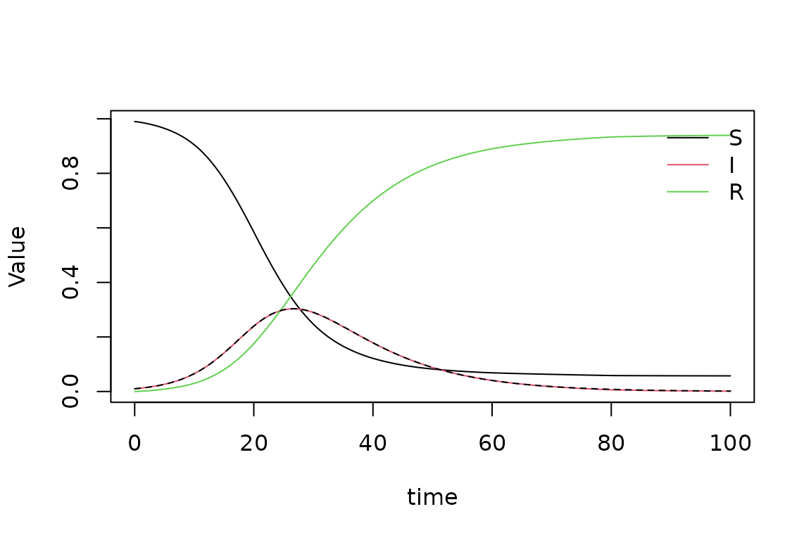

2. Estimating parameters from data

Suppose we only observe the infected and recovered fractions every five days, with measurement noise, and want to estimate beta and gamma.

set.seed(42)
obs <- ref[ref$time %% 5 == 0, c("time", "I", "R")]
obs$I <- obs$I + rnorm(nrow(obs), sd = 0.005)
obs$R <- obs$R + rnorm(nrow(obs), sd = 0.005)
head(obs)
#>    time          I            R
#> 1     0 0.01685479 -0.008906542
#> 6     5 0.02353904  0.007607310
#> 11   10 0.06721241  0.036184205
#> 16   15 0.14465968  0.089668878
#> 21   20 0.24189748  0.173530409
#> 26   25 0.29943608  0.312187441

Give starting guesses in unknown and the observations in data. The derivative function is unchanged; beta and gamma are now learned.

inv <- pinn_ode(sir, y0 = y0, times = times,
                unknown = c(beta = 0.5, gamma = 0.2), data = obs)
fit_inv <- pinn_fit(inv, epochs = 5000, seed = 1)
coef(fit_inv)
#>       beta      gamma 
#> 0.29416921 0.09781107

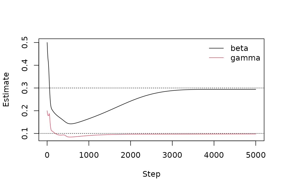
The true values are beta = 0.3 and gamma = 0.1. The estimates’ path during training is useful for judging convergence:

plot(fit_inv, type = "parameters")
abline(h = c(0.3, 0.1), lty = 3)

Observations do not have to cover every state: here S was never observed. Missing values (NA) in data are also ignored, so different states can be measured at different times.

3. Solving a PDE

For PDEs, describe the domain, the residual and the conditions directly. The residual is an ordinary R function whose arguments are matched by name to outputs (u), variables (x, t) and parameters (a). The function d() takes derivatives: d(u, t) is $\partial u/\partial t$ and d(u, x, x) is $\partial^2 u / \partial x^2$ .

The heat equation $u_t = a\,u_{xx}$ on $0 \le x \le 1$ , with $u(x, 0) = \sin(\pi x)$ and $u = 0$ at both ends, has the exact solution $u = e^{-a\pi^2 t}\sin(\pi x)$ .

heat <- pinn_problem(
  domain = pinn_domain(x = c(0, 1), t = c(0, 1)),
  outputs = "u",
  residual = function(u, x, t, a, d) d(u, t) - a * d(u, x, x),
  conditions = list(
    pinn_initial(function(x) sin(pi * x), time = "t"),
    pinn_dirichlet(where = list(x = "both"), value = 0)
  ),
  parms = list(a = 0.1)
)
fit_heat <- pinn_fit(heat, epochs = 5000, seed = 1)

grid <- expand.grid(x = seq(0, 1, length.out = 51), t = seq(0, 1, length.out = 51))
pred <- predict(fit_heat, grid)
max(abs(pred$u - exp(-0.1 * pi^2 * grid$t) * sin(pi * grid$x)))
#> [1] 0.006326235
plot(fit_heat, type = "solution")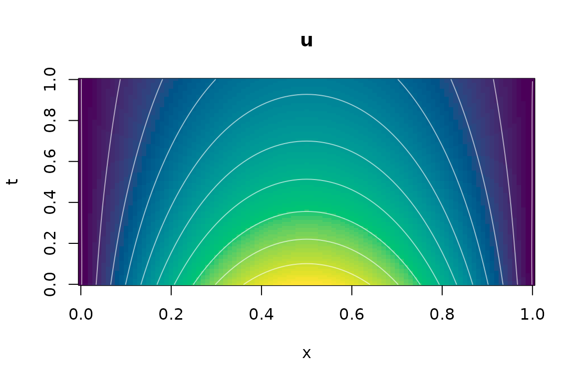

residuals() shows where the equation is satisfied least well, which is a useful diagnostic when no exact solution is available:

res <- residuals(fit_heat, grid)
summary(abs(res$residual_u))
#>      Min.   1st Qu.    Median      Mean   3rd Qu.      Max. 
#> 9.127e-06 4.437e-03 5.434e-03 5.858e-03 6.983e-03 4.144e-02

Tips

Write tensor-friendly code. Inside residual, condition and ODE functions the arguments are torch tensors. Arithmetic and functions such as sin, exp, log and sqrt work; if, ifelse, max and pmin on these values do not.
When the loss stalls, try more epochs, a larger network (hidden), more collocation points (n_collocation), or follow Adam with L-BFGS (lbfgs_iter = 500). plot(fit) shows the loss history.
Scale your problem. PINNs train best when inputs and outputs are of order one. Inputs are rescaled automatically; rescale outputs that are very large or small.
Saving. Use pinn_save() and pinn_load(), because torch modules cannot be saved with saveRDS() alone.
Hardware. Pass device = "cuda" or device = "mps" to train on a GPU.